Abstract
tidymodels ist das R-Ökosystem für maschinelles Lernen im Tidyverse-Stil: deklarativ, modular und reproduzierbar. Es ersetzt das ältere caret-Paket durch eine Familie spezialisierter Pakete – rsample für Resampling, recipes für Feature-Engineering, parsnip für Modellspezifikation, tune für Hyperparameter-Optimierung und yardstick für Metriken. Für Bioinformatik-Teams, die ihre Analyse-Pipelines in R aufbauen und Wert auf saubere, nachvollziehbare Workflows legen, ist tidymodels die modernste Option.
Typisches Projektszenario
Ein Biomarker-Forschungsteam entwickelt ein prognostisches Modell für das Rückfallrisiko bei Brustkrebs-Patientinnen anhand eines 70-Gen-Panels (MammaPrint-ähnlich). Die Eingabedaten: normalisierte Expressionswerte von 70 Genen × 450 Patientinnen (280 rückfallfrei, 170 mit Rezidiv innerhalb von 5 Jahren). Ziel: ein robustes binäres Klassifikationsmodell, das AUC > 0.85 in 10-facher Kreuzvalidierung erreicht, mit interpretierbaren Feature-Importanzen für die klinische Diskussion.
Welches Problem löst tidymodels?
- Fragmentierte ML-Landschaft in R: Jedes ML-Paket in R hat seine eigene API (randomForest, glmnet, xgboost, ranger). tidymodels abstrahiert diese hinter einer einheitlichen Schnittstelle –
parsnip::set_engine()wählt das Backend, die Analyse-Logik bleibt identisch. - Reproduzierbares Feature-Engineering:
recipesdefiniert Vorverarbeitungsschritte (Normalisierung, Imputation, PCA, Interaktionen) als deklaratives Rezept, das innerhalb der Resampling-Schleife angewendet wird – Data-Leakage wird strukturell verhindert. - Saubere Hyperparameter-Optimierung:
tune+dialsbieten Grid-Search, Random Search und Bayesian Optimization mit konsistenter Ergebnis-Struktur.
Warum Teams tidymodels einsetzen
- Tidyverse-Integration: Pipes (
%>%/|>), tibbles, ggplot2 – tidymodels fügt sich nahtlos in bestehende R-Workflows ein. - Workflow-Objekt:
workflow()bündelt Rezept + Modell in einem einzigen Objekt, das gefittet, getunt und evaluiert werden kann – das Pendant zu sklearnsPipeline. - Modellwechsel in einer Zeile: Durch das Parsnip-Interface kann das Modell gewechselt werden, ohne den Rest der Pipeline zu ändern (
set_engine("ranger")→set_engine("xgboost")). - Metrik-Konsistenz: yardstick bietet über 50 Metriken mit einheitlicher API – von ROC-AUC über Brier-Score bis zu Concordance Index.
- Workflowsets:
workflow_set()vergleicht systematisch mehrere Modell-Rezept-Kombinationen in einem Experiment.
Das Workflow-Konzept
tidymodels trennt das Machine-Learning-Problem in klar definierte Schichten, die zusammen den Workflow bilden. Das Recipe (recipes-Paket) beschreibt, wie die Rohdaten transformiert werden: step_normalize() für Zentrierung/Skalierung, step_impute_knn() für fehlende Werte, step_pca() für Dimensionsreduktion, step_corr() zum Entfernen stark korrelierter Features. Jeder Schritt wird nur auf den Trainingsdaten "gelernt" und dann auf die Testdaten angewendet – das verhindert Data-Leakage strukturell.
Das Modell (parsnip-Paket) wird engine-agnostisch spezifiziert: logistic_reg(penalty = tune(), mixture = 1) definiert eine LASSO-Regression, ohne das Backend zu fixieren. Erst set_engine("glmnet") wählt die Implementierung. Das ermöglicht später den Wechsel zu "LiblineaR" oder "stan" ohne Änderung am Rest.
Das Tuning (tune-Paket) füllt die mit tune() markierten Platzhalter. tune_grid() evaluiert ein Parametersgitter über Resampling-Folds, tune_bayes() nutzt Bayesian Optimization mit Gaussian-Process-Surrogaten. Die Ergebnisse werden als ordentliches Tibble zurückgegeben – filterbar, plottbar, vergleichbar.
R-Code: tidymodels-Pipeline
library(tidymodels)
library(finetune)
tidymodels_prefer()

# Daten laden
breast <- read_csv("breast_70gene.csv") |>
  mutate(recurrence = factor(recurrence, levels = c("no","yes")))

# Resampling-Strategie
set.seed(42)
folds <- vfold_cv(breast, v = 10, strata = recurrence)

# Rezept: Vorverarbeitung
rec <- recipe(recurrence ~ ., data = breast) |>
  step_normalize(all_numeric_predictors()) |>
  step_corr(all_numeric_predictors(), threshold = 0.9) |>
  step_zv(all_predictors())

# Modell: XGBoost mit tuning-Platzhaltern
xgb_spec <- boost_tree(
  trees = tune(),
  tree_depth = tune(),
  learn_rate = tune(),
  min_n = tune()
) |>
  set_engine("xgboost") |>
  set_mode("classification")

# Workflow
wf <- workflow() |>
  add_recipe(rec) |>
  add_model(xgb_spec)

# Hyperparameter-Tuning (Bayesian)
xgb_params <- extract_parameter_set_dials(wf) |>
  update(trees = trees(range = c(100, 1000)),
         tree_depth = tree_depth(range = c(2, 8)))

bayes_res <- tune_bayes(
  wf, resamples = folds,
  param_info = xgb_params,
  initial = 10, iter = 30,
  metrics = metric_set(roc_auc, accuracy, brier_class),
  control = control_bayes(verbose = TRUE, no_improve = 10)
)

# Bestes Modell finalisieren
best <- select_best(bayes_res, metric = "roc_auc")
final_wf <- finalize_workflow(wf, best)
final_fit <- fit(final_wf, breast)

# Feature Importance
library(vip)
final_fit |>
  extract_fit_engine() |>
  vip(num_features = 20)
Beispielausgabe
# 10-fold CV Results (best):
# roc_auc = 0.891  accuracy = 0.824  brier_class = 0.134

# Best hyperparameters:
# trees = 487, tree_depth = 4, learn_rate = 0.032, min_n = 8

# Top 10 features by importance:
# 1. CCNE2    (Cell Cycle)
# 2. MMP9     (Invasion)
# 3. VEGFA    (Angiogenesis)
# 4. ESR1     (Hormone Receptor)
# 5. AURKA    (Mitosis)
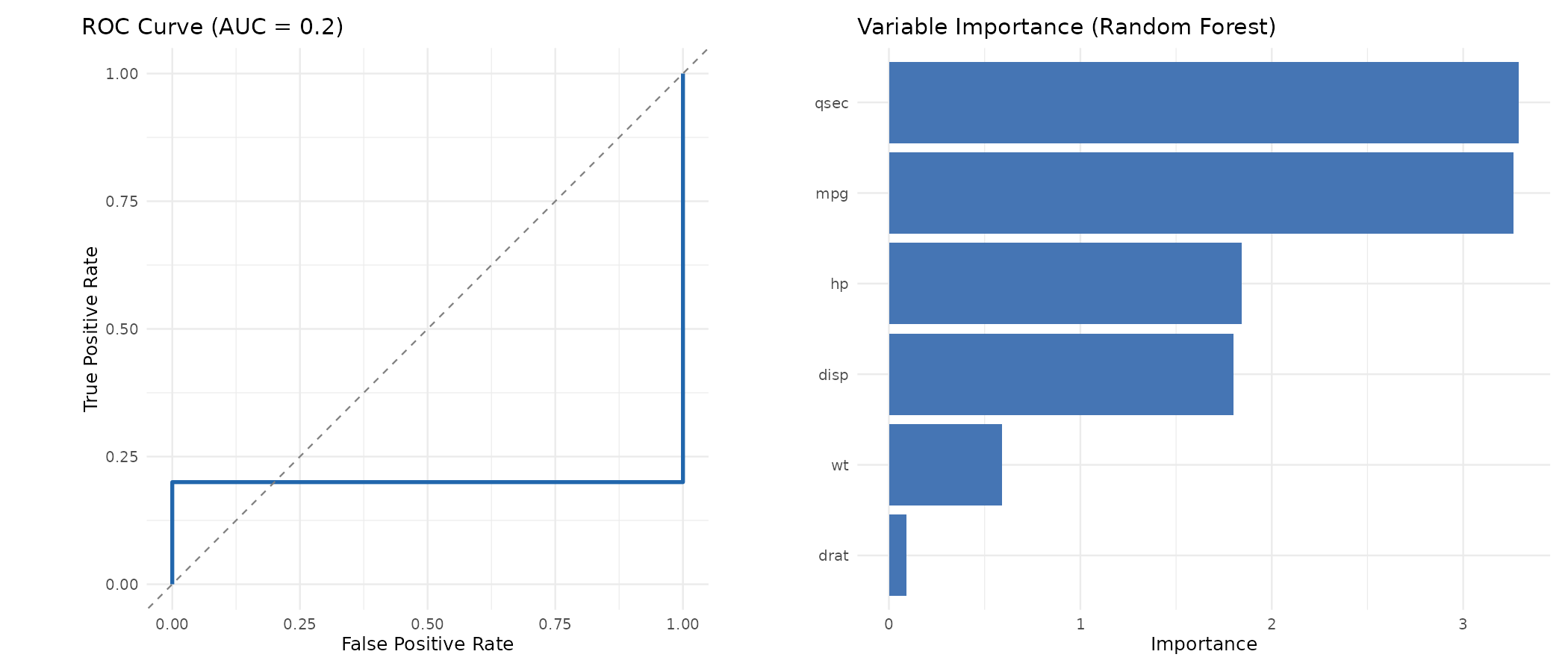
Diagnostische Plots
Vergleich mit Alternativen
| Merkmal | tidymodels | caret | mlr3 | sklearn |
|---|---|---|---|---|
| Sprache | R | R | R | Python |
| Designphilosophie | Tidyverse (deklarativ) | Prozedural | R6 (OOP) | OOP + funktional |
| Preprocessing | recipes (deklarativ) | preProcess | mlr3pipelines | Pipeline + Transformer |
| Tuning | tune + finetune | trainControl | mlr3tuning | GridSearchCV |
| Bayesian Tuning | tune_bayes() | Nicht nativ | mlr3mbo | Extern (optuna) |
| Modellvergleich | workflow_set() | resamples() | benchmark() | Manuell |
| Maintenance | Aktiv (Posit/RStudio) | Wenig aktiv | Aktiv | Sehr aktiv |
Statistische Vertiefung
Die Bayesian Optimization in tune_bayes() nutzt einen Gaussian-Process-Surrogaten, um die teure Zielfunktion (Modelltraining + CV-Evaluation) effizient zu approximieren. Im Vergleich zu Grid-Search, das exponentiell mit der Parameteranzahl wächst, benötigt Bayesian Optimization typisch 30–50 Evaluationen für 4–6 Hyperparameter – ein Faktor-10-Speedup gegenüber vollständigem Grid-Search. Die Acquisition-Funktion (Expected Improvement) balanciert Exploration (unbekannte Regionen) und Exploitation (vielversprechende Regionen).
Der Brier-Score als ergänzende Metrik zur ROC-AUC misst die Kalibrierung der vorhergesagten Wahrscheinlichkeiten. Ein Modell mit hoher AUC kann schlecht kalibriert sein, wenn es z.B. Wahrscheinlichkeiten von 0.95 vorhersagt, obwohl die wahre Rate nur 0.70 beträgt. Für klinische Entscheidungen ist die Kalibrierung oft wichtiger als die Diskrimination – ein Patient möchte wissen, ob sein Risiko 30% oder 70% beträgt, nicht nur ob es "hoch" oder "niedrig" ist.
Die Feature-Importance-Analyse über das vip-Paket bietet modellabhängige (Gain, Cover, Frequency für Baummodelle) und modellunabhängige (Permutation Importance) Methoden. Permutation Importance ist robuster, da sie den tatsächlichen Leistungsverlust bei Permutation eines Features misst – Gain kann bei korrelierten Features irreführend sein, weil der Beitrag auf mehrere korrelierte Features aufgeteilt wird.
Zitationen
- Kuhn M, Wickham H (2020). Tidy Modeling with R. O’Reilly Media. tmwr.org
- Kuhn M, Silge J (2022). “tidymodels: a collection of packages for modeling and machine learning using tidyverse principles.” tidymodels.org
- Brier GW (1950). “Verification of forecasts expressed in terms of probability.” Monthly Weather Review, 78(1), 1–3.
Fazit
tidymodels ist die eleganteste ML-Plattform in R. Die deklarative Syntax, die strukturelle Verhinderung von Data-Leakage und die nahtlose Tidyverse-Integration machen es zur idealen Wahl für Teams, die bereits im R-Ökosystem arbeiten. Limitierungen: (1) Langsamere Ausführung als sklearn bei großen Datensätzen (R-Overhead). (2) Weniger Community-Ressourcen als sklearn (Stack Overflow, Tutorials). (3) GPU-Support nur über externe Engines (torch). Aber für klinische Biomarker-Studien mit überschaubaren Datengrößen bietet tidymodels die sauberste und reproduzierbarste Pipeline.
Dokumentation
Abstract
tidymodels is the R ecosystem for machine learning in tidyverse style: declarative, modular, and reproducible. It replaces the older caret package with a family of specialized packages—rsample for resampling, recipes for feature engineering, parsnip for model specification, tune for hyperparameter optimization, and yardstick for metrics. For bioinformatics teams building their analysis pipelines in R and valuing clean, traceable workflows, tidymodels is the most modern option.
Typical Project Scenario
A biomarker research team develops a prognostic model for breast cancer recurrence risk using a 70-gene panel (MammaPrint-like). Input data: normalized expression values from 70 genes × 450 patients (280 recurrence-free, 170 with recurrence within 5 years). Goal: a robust binary classification model achieving AUC > 0.85 in 10-fold cross-validation, with interpretable feature importances for clinical discussion.
What Problem Does tidymodels Solve?
- Fragmented ML landscape in R: Every ML package in R has its own API (randomForest, glmnet, xgboost, ranger). tidymodels abstracts these behind a unified interface—
parsnip::set_engine()selects the backend while analysis logic remains identical. - Reproducible feature engineering:
recipesdefines preprocessing steps (normalization, imputation, PCA, interactions) as a declarative recipe applied within the resampling loop—structurally preventing data leakage. - Clean hyperparameter optimization:
tune+dialsoffer grid search, random search, and Bayesian optimization with consistent result structures.
Why Teams Choose tidymodels
- Tidyverse integration: Pipes (
%>%/|>), tibbles, ggplot2—tidymodels fits seamlessly into existing R workflows. - Workflow object:
workflow()bundles recipe + model into a single object that can be fitted, tuned, and evaluated—the counterpart to sklearn’sPipeline. - Model swapping in one line: Through the parsnip interface, models can be swapped without changing the rest of the pipeline (
set_engine("ranger")→set_engine("xgboost")). - Metric consistency: yardstick provides over 50 metrics with a unified API—from ROC-AUC through Brier score to concordance index.
- Workflowsets:
workflow_set()systematically compares multiple model-recipe combinations in one experiment.
The Workflow Concept
tidymodels separates the machine learning problem into clearly defined layers that together form the workflow. The Recipe (recipes package) describes how raw data is transformed: step_normalize() for centering/scaling, step_impute_knn() for missing values, step_pca() for dimensionality reduction, step_corr() for removing highly correlated features. Each step is "learned" only on training data and then applied to test data—structurally preventing data leakage.
The Model (parsnip package) is specified engine-agnostically: logistic_reg(penalty = tune(), mixture = 1) defines a LASSO regression without fixing the backend. Only set_engine("glmnet") selects the implementation—enabling later switches to "LiblineaR" or "stan" without changing the rest.
Tuning (tune package) fills placeholders marked with tune(). tune_grid() evaluates a parameter grid across resampling folds, tune_bayes() uses Bayesian optimization with Gaussian process surrogates. Results are returned as tidy tibbles—filterable, plottable, comparable.
R Code: tidymodels Pipeline
library(tidymodels)
library(finetune)
tidymodels_prefer()

# Load data
breast <- read_csv("breast_70gene.csv") |>
  mutate(recurrence = factor(recurrence, levels = c("no","yes")))

# Resampling strategy
set.seed(42)
folds <- vfold_cv(breast, v = 10, strata = recurrence)

# Recipe: preprocessing
rec <- recipe(recurrence ~ ., data = breast) |>
  step_normalize(all_numeric_predictors()) |>
  step_corr(all_numeric_predictors(), threshold = 0.9) |>
  step_zv(all_predictors())

# Model: XGBoost with tuning placeholders
xgb_spec <- boost_tree(
  trees = tune(),
  tree_depth = tune(),
  learn_rate = tune(),
  min_n = tune()
) |>
  set_engine("xgboost") |>
  set_mode("classification")

# Workflow
wf <- workflow() |>
  add_recipe(rec) |>
  add_model(xgb_spec)

# Hyperparameter tuning (Bayesian)
xgb_params <- extract_parameter_set_dials(wf) |>
  update(trees = trees(range = c(100, 1000)),
         tree_depth = tree_depth(range = c(2, 8)))

bayes_res <- tune_bayes(
  wf, resamples = folds,
  param_info = xgb_params,
  initial = 10, iter = 30,
  metrics = metric_set(roc_auc, accuracy, brier_class),
  control = control_bayes(verbose = TRUE, no_improve = 10)
)

# Finalize best model
best <- select_best(bayes_res, metric = "roc_auc")
final_wf <- finalize_workflow(wf, best)
final_fit <- fit(final_wf, breast)

# Feature importance
library(vip)
final_fit |>
  extract_fit_engine() |>
  vip(num_features = 20)
Example Output
# 10-fold CV Results (best):
# roc_auc = 0.891  accuracy = 0.824  brier_class = 0.134

# Best hyperparameters:
# trees = 487, tree_depth = 4, learn_rate = 0.032, min_n = 8

# Top 10 features by importance:
# 1. CCNE2    (Cell Cycle)
# 2. MMP9     (Invasion)
# 3. VEGFA    (Angiogenesis)
# 4. ESR1     (Hormone Receptor)
# 5. AURKA    (Mitosis)
Diagnostic Plots
Comparison with Alternatives
| Feature | tidymodels | caret | mlr3 | sklearn |
|---|---|---|---|---|
| Language | R | R | R | Python |
| Design philosophy | Tidyverse (declarative) | Procedural | R6 (OOP) | OOP + functional |
| Preprocessing | recipes (declarative) | preProcess | mlr3pipelines | Pipeline + Transformer |
| Tuning | tune + finetune | trainControl | mlr3tuning | GridSearchCV |
| Bayesian tuning | tune_bayes() | Not native | mlr3mbo | External (optuna) |
| Model comparison | workflow_set() | resamples() | benchmark() | Manual |
| Maintenance | Active (Posit/RStudio) | Low activity | Active | Very active |
Statistical Deep Dive
Bayesian optimization in tune_bayes() uses a Gaussian process surrogate to efficiently approximate the expensive objective function (model training + CV evaluation). Compared to grid search, which grows exponentially with parameter count, Bayesian optimization typically needs 30–50 evaluations for 4–6 hyperparameters—a 10× speedup over exhaustive grid search. The acquisition function (Expected Improvement) balances exploration (unknown regions) and exploitation (promising regions).
The Brier score as a complementary metric to ROC-AUC measures the calibration of predicted probabilities. A model with high AUC can be poorly calibrated if it predicts probabilities of 0.95 when the true rate is only 0.70. For clinical decisions, calibration is often more important than discrimination—a patient wants to know whether their risk is 30% or 70%, not just whether it is "high" or "low".
Feature importance analysis via the vip package offers model-dependent (Gain, Cover, Frequency for tree models) and model-independent (permutation importance) methods. Permutation importance is more robust since it measures the actual performance loss when permuting a feature—Gain can be misleading with correlated features because the contribution gets split across multiple correlated features.
Citations
- Kuhn M, Wickham H (2020). Tidy Modeling with R. O’Reilly Media. tmwr.org
- Kuhn M, Silge J (2022). “tidymodels: a collection of packages for modeling and machine learning using tidyverse principles.” tidymodels.org
- Brier GW (1950). “Verification of forecasts expressed in terms of probability.” Monthly Weather Review, 78(1), 1–3.
Conclusion
tidymodels is the most elegant ML platform in R. Its declarative syntax, structural prevention of data leakage, and seamless tidyverse integration make it ideal for teams already working in the R ecosystem. Limitations: (1) Slower execution than sklearn with large datasets (R overhead). (2) Fewer community resources than sklearn (Stack Overflow, tutorials). (3) GPU support only via external engines (torch). But for clinical biomarker studies with manageable data sizes, tidymodels offers the cleanest and most reproducible pipeline.