Abstract
Wenn ein Team in einem Omics-Projekt fragt, welche Gene oder miRNAs sich wirklich zwischen zwei Bedingungen unterscheiden, beginnt der schwierigste Teil nicht beim Plot, sondern bei der Statistik und dem Studiendesign. DESeq2 ist deshalb in vielen RNA-seq- und miRNA-Workflows ein Standard, weil es Count-Daten realistisch modelliert und die Unsicherheit transparent macht. Dieser Beitrag erzählt den Workflow aus der Perspektive eines Bioinformatikers in der Pipeline-Praxis: Problem, Moduswahl, Umsetzung, Interpretation, Limitationen und wissenschaftliche Einordnung.
Die typische Ausgangsszene im Projekt
Montagmorgen im Tumorboard-Projekt: Das Team hat neue Sequenzdaten, klinische Metadaten und eine klare Frage — welche molekularen Marker unterscheiden Responder und Non-Responder? Erste Tabellen sehen eindeutig aus, aber schnell tauchen Zweifel auf: unterschiedliche Library Sizes, Batch-Effekte, kleine Subgruppen, fehlende Covariates.
Genau hier wird DESeq2 relevant: Es hilft, beobachtete Unterschiede statistisch belastbar zu bewerten, statt visuelle Muster zu überinterpretieren.
Welches Problem löst das Package konkret?
- Technisches Problem: Count-Daten sind überdispers und nicht normalverteilt.
- Methodisches Problem: Viele Hypothesentests parallel erhöhen Fehlerrisiko.
- Interpretationsproblem: p-Werte ohne Effektgröße führen zu schwachen biologischen Aussagen.
DESeq2 adressiert diese drei Ebenen über Negativ-Binomial-Modellierung, FDR-Kontrolle und stabilisierte Effektgrößen (lfcShrink).
Warum nutzen Teams DESeq2 so häufig?
- Robuste Defaults für viele Bulk-RNA-seq-Szenarien
- Transparenter, gut dokumentierter Bioconductor-Workflow
- Gute Balance zwischen statistischer Strenge und praktischer Bedienbarkeit
- Hohe Anschlussfähigkeit an Pathway-/Enrichment- und Reporting-Workflows
Modes of Use: In welchen Modi man DESeq2 einsetzen kann
Mode 1 – Explorativ (Hypothesengenerierung)
Ziel: Kandidatengene/miRNAs identifizieren, Muster verstehen, Folgeexperimente planen. Schwellen werden transparent dokumentiert, aber nicht als endgültige Wahrheiten verkauft.
Mode 2 – Konfirmatorisch (präregistrierte Fragestellung)
Ziel: Vorab definierte Kontraste testen, striktere QC-Gates, saubere Kovariatenmodellierung, klarer Umgang mit Multiplen Tests.
Mode 3 – Pipeline/Produktion
Ziel: Reproduzierbare Runs in Snakemake/Nextflow, versionierte Inputs, automatisierte QC-Reports, standardisierte Outputs für kliniknahe Entscheidungswege.
Mode 4 – Python-integriert
Ziel: Nutzung über pyDESeq2 in Python-zentrierten MLOps-/Data-Engineering-Stacks, wenn R nicht die primäre Orchestrierungssprache ist.
R-Code (DESeq2) + Beispiel-Output
library(DESeq2)

dds <- DESeqDataSetFromMatrix(
  countData = countData,
  colData = colData,
  design = ~ batch + condition
)

keep <- rowSums(counts(dds) >= 10) >= 3
dds <- dds[keep, ]
dds <- DESeq(dds)

res <- results(dds, contrast = c("condition", "treated", "control"))
res_shrunk <- lfcShrink(dds, coef = "condition_treated_vs_control", type = "apeglm")

sig <- subset(as.data.frame(res_shrunk), padj < 0.05 & abs(log2FoldChange) >= 1)
Example output (demo):
Significant features: 248
Median abs(log2FC) among significant: 1.37
Python-Modus (pyDESeq2) + Beispiel-Output
from pydeseq2.dds import DeseqDataSet
from pydeseq2.ds import DeseqStats

dds = DeseqDataSet(
    counts=counts_df,
    metadata=metadata_df,
    design_factors=["batch", "condition"],
    refit_cooks=True,
)
dds.deseq2()

stats = DeseqStats(dds, contrast=["condition", "treated", "control"])
stats.summary()
results_df = stats.results_df
Example output (demo):
Converged fits: 2191 / 2200
Significant features (FDR<0.05): 271
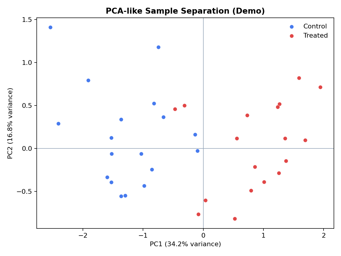
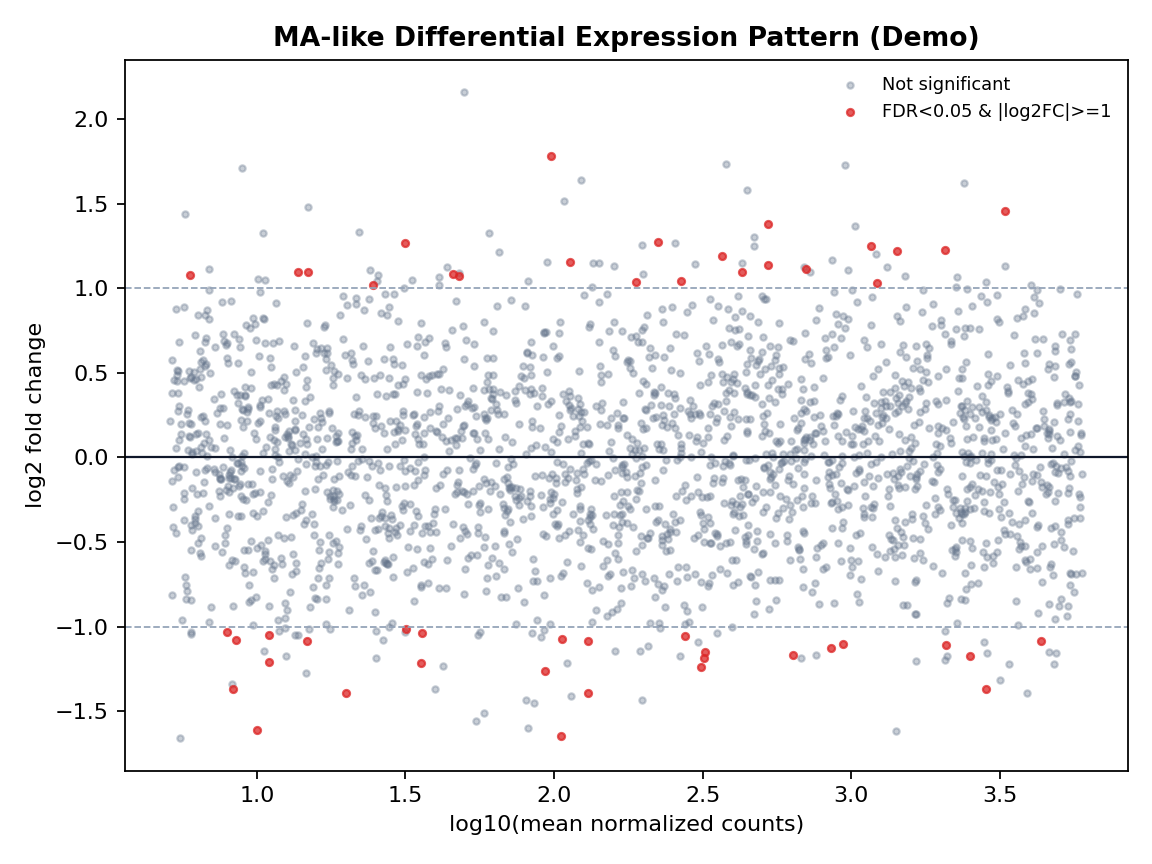
Eindrucksvolle Kernplots (Demo, reproduzierbar)
Vergleich mit Alternativen
| Kriterium | DESeq2 | edgeR | limma-voom |
|---|---|---|---|
| Modell | Negativ-Binomial | Negativ-Binomial | Lineares Modell nach voom |
| Stärke | Robuste Defaults | Sehr flexibel | Sehr effizient bei größeren Kohorten |
| miRNA-Use-Case | Gut bei sauberem Filtering | Sehr stark bei granularer Dispersion | Gut, wenn Annahmen passen |
Studien- und Literaturbezug (Citations)
DESeq2 wurde als methodischer Standard von Love, Huber und Anders eingeführt und breit in der RNA-seq-Praxis verankert. Für Workflow- und Methodenvergleich sind besonders folgende Arbeiten relevant:
- Love MI, Huber W, Anders S. Genome Biology (2014): DESeq2.
- Conesa A et al. Genome Biology (2016): Best practices für RNA-seq data analysis.
- Soneson C, Robinson MD. F1000Research (2018): Differential expression analysis review.
- Law CW et al. Genome Biology (2014): voom.
- Robinson MD, McCarthy DJ, Smyth GK. Bioinformatics (2010): edgeR.
Runder Abschluss: Kontext, Nutzen, Limitationen
Sinnvoller Kontext: Bulk-RNA-seq und miRNA-seq mit klarer experimenteller Frage, guter Metadatenqualität und reproduzierbarer Pipeline.
Gelöstes Problem: Belastbare DE-Inferenz statt bloßem Fold-Change-Vergleich.
Limitationen: Kleine Stichproben, fehlerhafte Designformeln, nicht adressierte Batch-Effekte und die Grenze zwischen Assoziation und Kausalität.
Manuals / Docs
Abstract
In omics projects, the hardest step is not producing a plot but deciding whether an observed expression change is biologically credible. DESeq2 became a default in many RNA-seq and miRNA workflows because it models count data realistically and quantifies uncertainty. This article tells the package story from a bioinformatics pipeline perspective: the problem, why teams choose it, operating modes, scientific evidence, and practical limitations.
A realistic project starting point
Imagine a translational study meeting: a team has new sequencing runs and asks which markers separate responders from non-responders. Early summary tables look convincing, then concerns appear — unequal library sizes, hidden batch effects, and small subgroup sizes. This is where DESeq2 matters: it helps separate robust signal from technical artifacts before clinical or biological interpretation.
What problem does DESeq2 solve?
- Technical: count data are overdispersed and not Gaussian.
- Statistical: thousands of parallel tests inflate false discoveries.
- Interpretation: p-values without effect sizes are weak evidence.
DESeq2 addresses all three through Negative Binomial modeling, FDR control, and stabilized log2 fold changes.
Why people use it in practice
- Strong defaults for many bulk RNA-seq study designs
- Transparent Bioconductor documentation and community practice
- Good trade-off between rigor and operational usability
- Easy integration with downstream pathway and reporting tools
Modes of use
Mode 1 – Exploratory
Generate hypotheses and prioritize candidates while documenting uncertainty.
Mode 2 – Confirmatory
Predefined contrasts, stricter QC gates, explicit covariate handling.
Mode 3 – Production pipeline
Snakemake/Nextflow orchestration with versioned inputs, automated QC, and standardized outputs.
Mode 4 – Python-native integration
Use via pyDESeq2 in Python-centric analytics and engineering stacks.
R implementation + sample output
res <- results(dds, contrast = c("condition", "treated", "control"))
res_shrunk <- lfcShrink(dds, coef = "condition_treated_vs_control", type = "apeglm")
Example output (demo):
Significant features: 248
Median abs(log2FC): 1.37
Python integration + sample output
stats = DeseqStats(dds, contrast=["condition", "treated", "control"])
stats.summary()
Example output (demo):
Converged fits: 2191 / 2200
Significant features (FDR<0.05): 271
High-impact plots for interpretation
Alternatives and when to choose them
| Criterion | DESeq2 | edgeR | limma-voom |
|---|---|---|---|
| Core model | Negative Binomial | Negative Binomial | Linear model after voom |
| Strength | Robust defaults | High flexibility | Efficient in larger cohorts |
| miRNA scenarios | Strong with careful filtering | Very strong with fine dispersion control | Good when assumptions hold |
Evidence and citations
- Love MI, Huber W, Anders S. Genome Biology (2014) – DESeq2.
- Conesa A et al. Genome Biology (2016) – RNA-seq best practices.
- Soneson C, Robinson MD. F1000Research (2018) – differential expression review.
- Law CW et al. Genome Biology (2014) – voom.
- Robinson MD, McCarthy DJ, Smyth GK. Bioinformatics (2010) – edgeR.
Rounded conclusion: context, value, limitations
Best context: Bulk RNA-seq and miRNA-seq studies with explicit design formulas and reproducible pipeline execution.
Problem solved: robust DE inference beyond naive fold-change comparisons.
Key limitations: small n, misspecified models, unresolved batch effects, and the association-vs-causation boundary.
Manuals / docs
Statistische Tiefenschicht: Warum die Schätzungen belastbar sind
DESeq2 modelliert Roh-Counts mit einer Negativ-Binomial-Verteilung und trennt damit zwei Dinge, die in RNA-seq zentral sind: den systematischen Mittelwert-Unterschied zwischen Bedingungen und die stochastische Überdispersion zwischen biologischen Replikaten. Genau diese Trennung macht die Inferenz robuster als naive Vergleiche auf transformierten TPM-Werten.
1) Normalisierung als Skalierungsproblem
Die Size-Factor-Schätzung (Median-of-Ratios) nimmt an, dass die Mehrheit der Gene nicht stark differentiell exprimiert ist. Für jedes Sample wird ein globaler Skalierungsfaktor geschätzt, sodass Bibliothekstiefen- und Kompositionsunterschiede entfernt werden, ohne ein einzelnes Referenzgen vorzuschreiben. Praktisch bedeutet das: Fold-Changes sind näher an biologischen Effekten und weniger an Sequenziertiefe gekoppelt.
2) Dispersion: Gen-spezifisch + Information aus der Gesamtheit
Für jedes Gen wird eine Rohdispersion geschätzt, dann auf eine Mean-Dispersion-Trendkurve geschrumpft (Empirical Bayes). Gene mit wenig Information werden stärker zur Trendkurve gezogen; Gene mit klarer Evidenz bleiben individueller. Dieser Bias-Varianz-Kompromiss reduziert instabile Extremwerte und verbessert Reproduzierbarkeit in kleinen Kohorten.
3) Wald-Test vs. Likelihood-Ratio-Test (LRT)
- Wald-Test: prüft gezielte Kontraste (z. B. Treatment vs Control) und ist ideal für präzise, vorab definierte Hypothesen.
- LRT: vergleicht verschachtelte Modelle und testet, ob ein ganzer Effektblock (z. B. Zeitverlauf, Interaktion) signifikant zum Modell beiträgt.
In explorativen Designs ist LRT oft informativer; in confirmatorischen Fragestellungen bleibt der Wald-Test meist die erste Wahl.
4) Log2 Fold-Change Shrinkage
Sehr niedrige Counts führen zu stark schwankenden Effektgrößen. Shrinkage-Methoden (z. B. apeglm) stabilisieren LFC-Schätzungen, ohne starke Signale übermäßig zu dämpfen. Dadurch werden Ranking, Priorisierung und Downstream-Interpretation (Pathways, Biomarkerlisten) deutlich belastbarer.
5) Multiple Tests, FDR und Power
Bei zehntausenden Genen ist unadjustiertes p-Value-Reporting statistisch unbrauchbar. DESeq2 nutzt FDR-Kontrolle (Benjamini-Hochberg) und unabhängiges Filtering, um die Entdeckungsrate unter Kontrolle zu halten und zugleich Power zu erhöhen. Für die Praxis heißt das: weniger falsche Treffer bei vergleichbarer Sensitivität.
Take-away für Omics-Teams
Wenn ein Team „belastbare Evidenz“ fordert, ist der entscheidende Punkt nicht nur ein schöner Volcano-Plot, sondern die Validität der Modellannahmen, die Stabilität der Effektgrößen und die saubere FDR-Kontrolle. Genau hier spielt DESeq2 seine Stärke aus.
Statistical Deep Layer: Why the estimates are trustworthy
DESeq2 models raw counts with a Negative Binomial distribution, explicitly separating condition-specific mean shifts from biological overdispersion. This separation is the key reason why inference is typically more robust than naive comparisons on transformed TPM values.
1) Normalization as a scaling problem
The median-of-ratios size-factor strategy assumes that most genes are not strongly differentially expressed. It estimates one global scaling factor per sample, removing library depth and composition effects without relying on a single reference gene. In practice, fold changes become less sequencing-depth-driven and more biologically interpretable.
2) Dispersion: gene-wise + pooled information
DESeq2 first estimates raw gene-wise dispersion, then shrinks it toward a mean-dispersion trend via empirical Bayes. Low-information genes borrow more strength from the global trend, while high-information genes remain more individual. This bias-variance tradeoff reduces unstable extremes and improves reproducibility in small cohorts.
3) Wald test vs. likelihood-ratio test (LRT)
- Wald test: best for targeted contrasts (e.g., treatment vs control) and pre-specified hypotheses.
- LRT: compares nested models and tests whether an entire effect block (e.g., time, interaction) contributes significantly.
LRT is often more informative in exploratory settings, while Wald remains a strong default in confirmatory analyses.
4) Log2 fold-change shrinkage
Very low counts can produce noisy and inflated effect-size estimates. Shrinkage methods (e.g., apeglm) stabilize LFC values without suppressing strong signals too aggressively. This leads to better ranking, prioritization, and downstream interpretation (pathways, candidate biomarkers).
5) Multiple testing, FDR, and statistical power
With tens of thousands of genes, raw p-values are not decision-ready. DESeq2 applies FDR control (Benjamini-Hochberg) and independent filtering to control false discoveries while improving power. Operationally, this means fewer false positives at comparable sensitivity.
Take-away for omics teams
When teams ask for “decision-grade evidence,” the decisive factors are not visual aesthetics but valid model assumptions, stable effect sizes, and disciplined FDR control. This is exactly where DESeq2 provides value.
Methodenwahl nach Datentyp: Welche Statistik wann Sinn macht
In der Praxis ist nicht die Frage „Welche Software ist die beste?“, sondern: Welches statistische Modell passt zur Daten-Generierungslogik? Ein Count-Modell ist nur dann stark, wenn die Annahmen zum biologischen und technischen Prozess passen.
1) Bulk RNA-seq mit biologischen Replikaten (typischer DE-Fall)
Für klassische Differential-Expression mit integer Counts und moderater Replikatzahl sind Negativ-Binomial-Modelle wie DESeq2 und edgeR die robusteste Standardwahl. Die Grundbelege stammen aus den methodischen Kernarbeiten zu DESeq2 (Love et al., 2014) und edgeR (Robinson et al., 2010), die zeigen, dass Dispersion korrekt modelliert und Unsicherheit bei kleinen n besser abgebildet wird als mit einfachen Poisson-/Normalannahmen.
2) Bulk RNA-seq mit komplexem Design (Batch, Kovariaten, Interaktionen)
Wenn das Design stark durch Kovariaten geprägt ist (z. B. Alter, RIN, Zentrum, Batch), bleiben GLM-basierte Ansätze sinnvoll. DESeq2 (Wald/LRT) und edgeR-GLM sind geeignet; bei sehr großen Designs wird häufig limma-voom genutzt, weil das lineare Modell mit Precision Weights flexibel für Kontrast- und Blocking-Strukturen ist (Law et al., 2014; Ritchie et al., 2015).
3) Kleine Effektgrößen + Ranking-fokussierte Priorisierung
Wenn biologisch kleine, aber konsistente Effekte relevant sind, ist LFC-Shrinkage wichtig (z. B. apeglm). Die Shrinkage-Literatur (Zhu et al., 2019) zeigt, dass stabilisierte Effektgrößen für Priorisierung und Reproduzierbarkeit nützlicher sind als rohe LFCs bei niedrigen Counts.
4) Transcript-/Isoform-Level statt Gen-Level
Für Isoform-Fragen ist ein reines Gen-Count-Modell oft zu grob. Best Practice ist heute quantifier-basiertes Transcript-Level mit gene-level summarization/offset-Strategien (z. B. tximport; Soneson, Love & Robinson, 2015). Für Differential Transcript Usage sind spezialisierte Verfahren (z. B. DEXSeq-ähnliche Frames) methodisch passender.
5) Single-cell RNA-seq (Zellniveau) vs. Pseudobulk
Auf Zellebene sind Zero-Inflation, Heterogenität und Pseudoreplikation zentrale Risiken. Viele Benchmarks empfehlen für robuste Gruppenvergleiche ein Pseudobulk-Design auf Sample-Ebene, wodurch klassische NB- oder limma-Frameworks wieder valide werden (z. B. Crowell et al., 2020). Zelllevel-Modelle wie MAST (Finak et al., 2015) sind nützlich für spezifische Fragestellungen, brauchen aber saubere Random-Effect/Donor-Strategien.
6) Compositional Omics (Mikrobiom) und relative Daten
Bei strikt compositionalen Daten sind absolute Count-Interpretationen gefährlich. Hier sind log-ratio-basierte oder compositional-aware Methoden methodisch angemessener als naives DE auf relativen Anteilen. Das ist ein anderer inferenzieller Raum als klassische Bulk RNA-seq DE.
7) Längsschnitt/Repeated Measures
Wenn dieselben Individuen mehrfach gemessen werden, muss die Korrelation innerhalb des Subjects explizit modelliert werden (Mixed-Effects oder Design-Matrizen mit geeigneten Block-Strukturen). Ein ignorierter Within-Subject-Zusammenhang produziert anti-konservative p-Werte.
Konkrete Entscheidungsregel für Teams
- Bulk RNA-seq, Standard-DE: DESeq2 oder edgeR.
- Komplexe Kontraste/Batch-reich: DESeq2-GLM oder limma-voom.
- Priorisierung bei kleinen Effekten: Shrinkage-LFC (apeglm).
- scRNA Gruppenvergleich: bevorzugt Pseudobulk pro Sample/Donor.
- Isoform-Frage: transcript-aware Workflow statt reines Genmodell.
Studien und methodische Kernquellen
- Love MI, Huber W, Anders S (2014). Moderated estimation of fold change and dispersion for RNA-seq data with DESeq2. Genome Biology.
- Robinson MD, McCarthy DJ, Smyth GK (2010). edgeR: a Bioconductor package for differential expression analysis of digital gene expression data. Bioinformatics.
- Law CW et al. (2014). voom: precision weights unlock linear model analysis tools for RNA-seq read counts. Genome Biology.
- Ritchie ME et al. (2015). limma powers differential expression analyses for RNA-sequencing and microarray studies. Nucleic Acids Research.
- Zhu A, Ibrahim JG, Love MI (2019). Heavy-tailed prior distributions for sequence count data: removing the noise and preserving large differences. Bioinformatics.
- Soneson C, Love MI, Robinson MD (2015). Differential analyses for RNA-seq: transcript-level estimates improve gene-level inferences. F1000Research.
- Finak G et al. (2015). MAST: a flexible statistical framework for assessing transcriptional changes and characterizing heterogeneity in single-cell RNA sequencing data. Genome Biology.
- Crowell HL et al. (2020). On the discovery of subpopulation-specific state transitions from multi-sample multi-condition single-cell RNA sequencing data. Nature Communications.
Method selection by data type: which statistics make sense when
In real projects, the key question is not “Which package is best?”, but which statistical model matches the data-generating process. A count model is only defensible when assumptions align with biology and measurement noise.
1) Bulk RNA-seq with biological replicates (standard DE setting)
For classical differential expression on integer counts with moderate replication, Negative Binomial frameworks (DESeq2, edgeR) remain the strongest default. Foundational work (Love et al., 2014; Robinson et al., 2010) demonstrates robust dispersion handling and better uncertainty quantification than naive Poisson/normal assumptions.
2) Complex bulk RNA-seq designs (batch, covariates, interactions)
When design complexity is high, GLM-based modeling is essential. DESeq2 (Wald/LRT) and edgeR-GLM are appropriate; limma-voom is often preferred for large contrast spaces because precision-weighted linear modeling handles blocking and flexible contrasts efficiently (Law et al., 2014; Ritchie et al., 2015).
3) Small effects and ranking-focused prioritization
When subtle but consistent biology matters, log2 fold-change shrinkage is critical (e.g., apeglm). The shrinkage literature (Zhu et al., 2019) shows improved effect-size stability and more reliable ranking for downstream prioritization.
4) Transcript/isoform-level questions
Pure gene-level count models can be too coarse for isoform biology. Transcript-aware workflows (e.g., tximport-style summarization/offsets) improve gene-level inference from transcript estimates (Soneson, Love & Robinson, 2015), while DTU questions need dedicated transcript-usage frameworks.
5) Single-cell RNA-seq: cell-level vs pseudobulk
Single-cell analyses face dropout, heterogeneity, and pseudo-replication risks. Many benchmark-style evaluations support pseudobulk aggregation at sample/donor level for robust group inference (e.g., Crowell et al., 2020), while cell-level models such as MAST (Finak et al., 2015) can be effective when donor structure is modeled correctly.
6) Compositional omics (microbiome) and relative data
For strictly compositional data, naive count-style interpretation on relative abundances is statistically fragile. Log-ratio or composition-aware models are typically more appropriate than direct transplantation of bulk RNA-seq DE logic.
7) Longitudinal/repeated-measures studies
Repeated sampling from the same subject requires explicit within-subject correlation modeling (mixed models or properly blocked designs). Ignoring this structure leads to anti-conservative p-values and inflated discoveries.
Practical decision rule for teams
- Bulk RNA-seq, standard DE: DESeq2 or edgeR.
- High-complexity contrasts: DESeq2-GLM or limma-voom.
- Ranking under low counts: shrinkage LFC (apeglm).
- scRNA group inference: prefer pseudobulk at donor/sample level.
- Isoform-level biology: transcript-aware workflow, not gene-only shortcuts.
Evidence base and core methodological sources
- Love MI, Huber W, Anders S (2014). Moderated estimation of fold change and dispersion for RNA-seq data with DESeq2. Genome Biology.
- Robinson MD, McCarthy DJ, Smyth GK (2010). edgeR: a Bioconductor package for differential expression analysis of digital gene expression data. Bioinformatics.
- Law CW et al. (2014). voom: precision weights unlock linear model analysis tools for RNA-seq read counts. Genome Biology.
- Ritchie ME et al. (2015). limma powers differential expression analyses for RNA-sequencing and microarray studies. Nucleic Acids Research.
- Zhu A, Ibrahim JG, Love MI (2019). Heavy-tailed prior distributions for sequence count data: removing the noise and preserving large differences. Bioinformatics.
- Soneson C, Love MI, Robinson MD (2015). Differential analyses for RNA-seq: transcript-level estimates improve gene-level inferences. F1000Research.
- Finak G et al. (2015). MAST: a flexible statistical framework for assessing transcriptional changes and characterizing heterogeneity in single-cell RNA sequencing data. Genome Biology.
- Crowell HL et al. (2020). On the discovery of subpopulation-specific state transitions from multi-sample multi-condition single-cell RNA sequencing data. Nature Communications.
Direktlinks zu den zitierten Studien (Open/Publisher Pages)
- Love et al. (2014) — DESeq2, Genome Biology
- Robinson et al. (2010) — edgeR, Bioinformatics
- Law et al. (2014) — voom, Genome Biology
- Ritchie et al. (2015) — limma, Nucleic Acids Research
- Zhu et al. (2019) — apeglm/LFC shrinkage, Bioinformatics
- Soneson et al. (2015) — transcript-level inference, F1000Research
- Finak et al. (2015) — MAST for single-cell RNA-seq, Genome Biology
- Crowell et al. (2020) — multi-sample single-cell state transitions, Nature Communications
Direct links to cited studies (open/publisher pages)
- Love et al. (2014) — DESeq2, Genome Biology
- Robinson et al. (2010) — edgeR, Bioinformatics
- Law et al. (2014) — voom, Genome Biology
- Ritchie et al. (2015) — limma, Nucleic Acids Research
- Zhu et al. (2019) — apeglm/LFC shrinkage, Bioinformatics
- Soneson et al. (2015) — transcript-level inference, F1000Research
- Finak et al. (2015) — MAST for single-cell RNA-seq, Genome Biology
- Crowell et al. (2020) — multi-sample single-cell state transitions, Nature Communications