Prolog: Die Landkarte der Regulatoren
Gene arbeiten nicht allein. Jedes Gen ist Teil eines Netzwerks aus Regulatoren, Targets und Feedback-Schleifen. In der Krebsbiologie sind es vor allem die miRNAs, die als Master-Regulatoren fungieren: Eine einzige miRNA kann Hunderte von Zielgenen gleichzeitig kontrollieren. Aber wie macht man diese unsichtbaren Beziehungen sichtbar? Die Antwort: Netzwerk-Graphen — mathematische Strukturen, in denen Knoten für Moleküle und Kanten für Interaktionen stehen.
In dieser Geschichte konstruieren wir ein miRNA-Target-Netzwerk für Brustkrebs und enthüllen Schritt für Schritt, wer die Schaltzentralen sind, welche Module zusammenarbeiten und wie sich das Netzwerk im Tumor verändert.
Kapitel 1: Das Netzwerk entsteht — miRNAs und ihre Targets
Unser Ausgangspunkt: Fünf Hub-miRNAs, die in der Brustkrebsbiologie eine zentrale Rolle spielen — miR-21, miR-155, miR-34a, miR-145 und miR-200c. Jede davon reguliert eine spezifische Gruppe von Zielgenen. Die Kanten des Netzwerks repräsentieren experimentell validierte miRNA-Target-Interaktionen aus Datenbanken wie miRTarBase und TargetScan.
Der erste Plot zeigt das Gesamtbild: Rote Diamanten sind miRNAs, blaue Kreise sind Zielgene. Die räumliche Anordnung (Spring-Layout) platziert stark verbundene Knoten näher zusammen. Sofort wird sichtbar, welche Gene von mehreren miRNAs gleichzeitig reguliert werden — das sind die Konvergenzpunkte des Netzwerks.
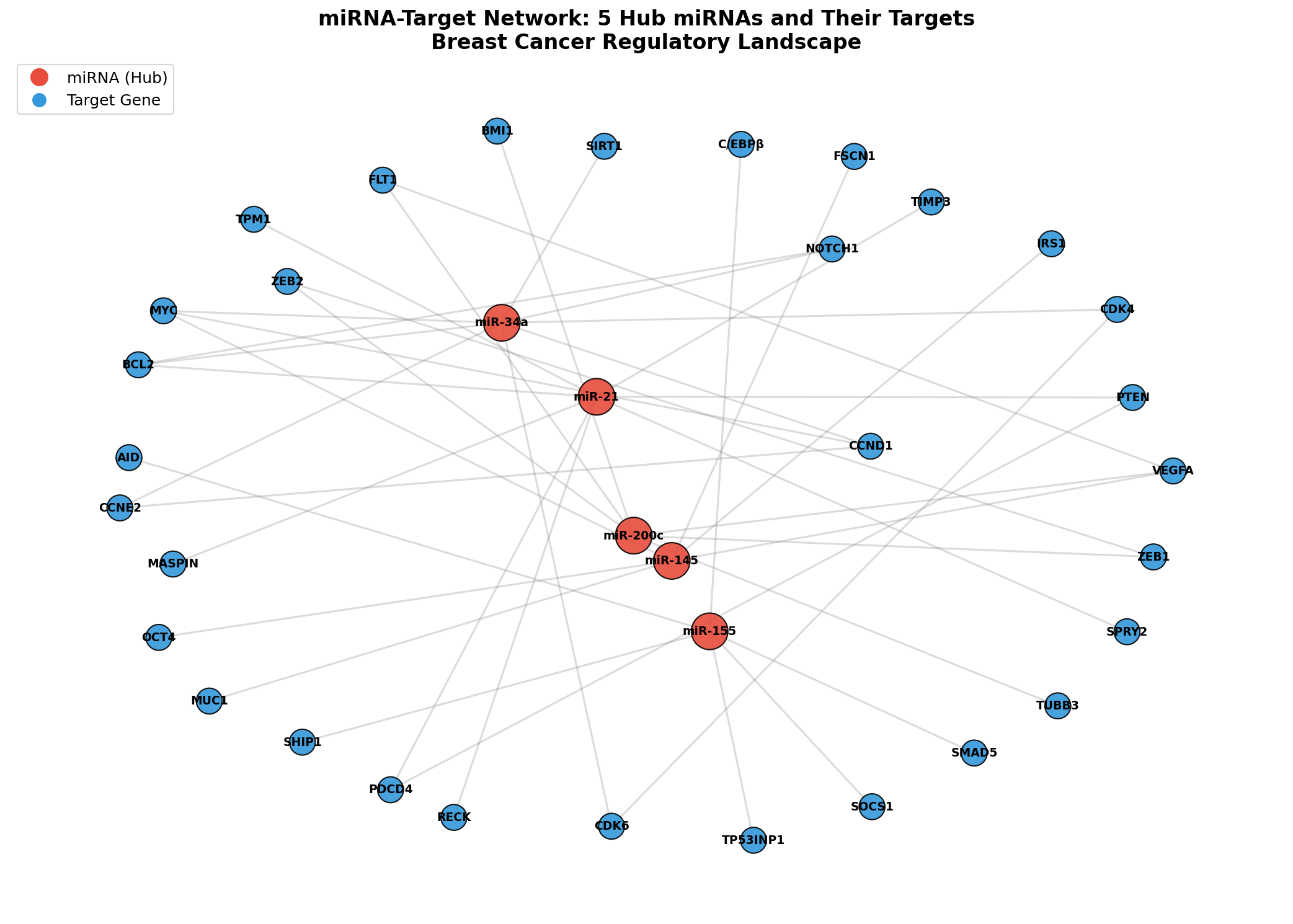
Das Grundnetzwerk zeigt bereits eine wichtige Erkenntnis: Die miRNA-Regulation ist nicht eins-zu-eins, sondern many-to-many. miR-21 reguliert 8 Targets, aber BCL2 wird sowohl von miR-21 als auch von miR-34a reguliert. Diese Redundanz macht das Netzwerk robust — der Ausfall einer einzelnen miRNA wird durch andere kompensiert.
Kapitel 2: Die Schaltzentralen — Grad-gewichtete Netzwerke
Nicht alle Knoten sind gleich wichtig. Der Grad (degree) eines Knotens — die Anzahl seiner Verbindungen — ist ein Maß für seinen Einfluss. Knoten mit vielen Verbindungen heißen Hubs. In biologischen Netzwerken folgt die Gradverteilung oft einem Power Law: Wenige Hubs haben extrem viele Verbindungen, während die Mehrheit der Knoten nur wenige hat.
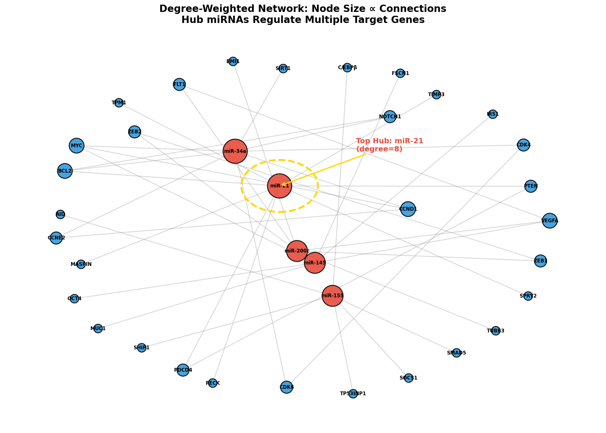
Die Hub-Analyse hat direkte therapeutische Relevanz: Wenn eine einzelne miRNA 8 Tumorsuppressor-Gene gleichzeitig unterdrückt (wie miR-21), dann ist die Inhibition dieser miRNA effizienter als die Aktivierung jedes einzelnen Targets. Das ist das Prinzip der Anti-miR-Therapie — und der Netzwerk-Graph zeigt, warum es funktioniert.
Kapitel 3: Funktionelle Module — Gemeinsam statt einsam
Biologische Netzwerke sind nicht zufällig verdrahtet — sie organisieren sich in Module: Gruppen von Knoten, die intern stark und extern schwach verbunden sind. Jedes Modul repräsentiert eine biologische Funktion. In unserem Netzwerk identifizieren wir vier Module: Zellzyklus (rot), Apoptose (blau), Epithelial-Mesenchymale Transition (EMT) (grün) und Angiogenese (orange).
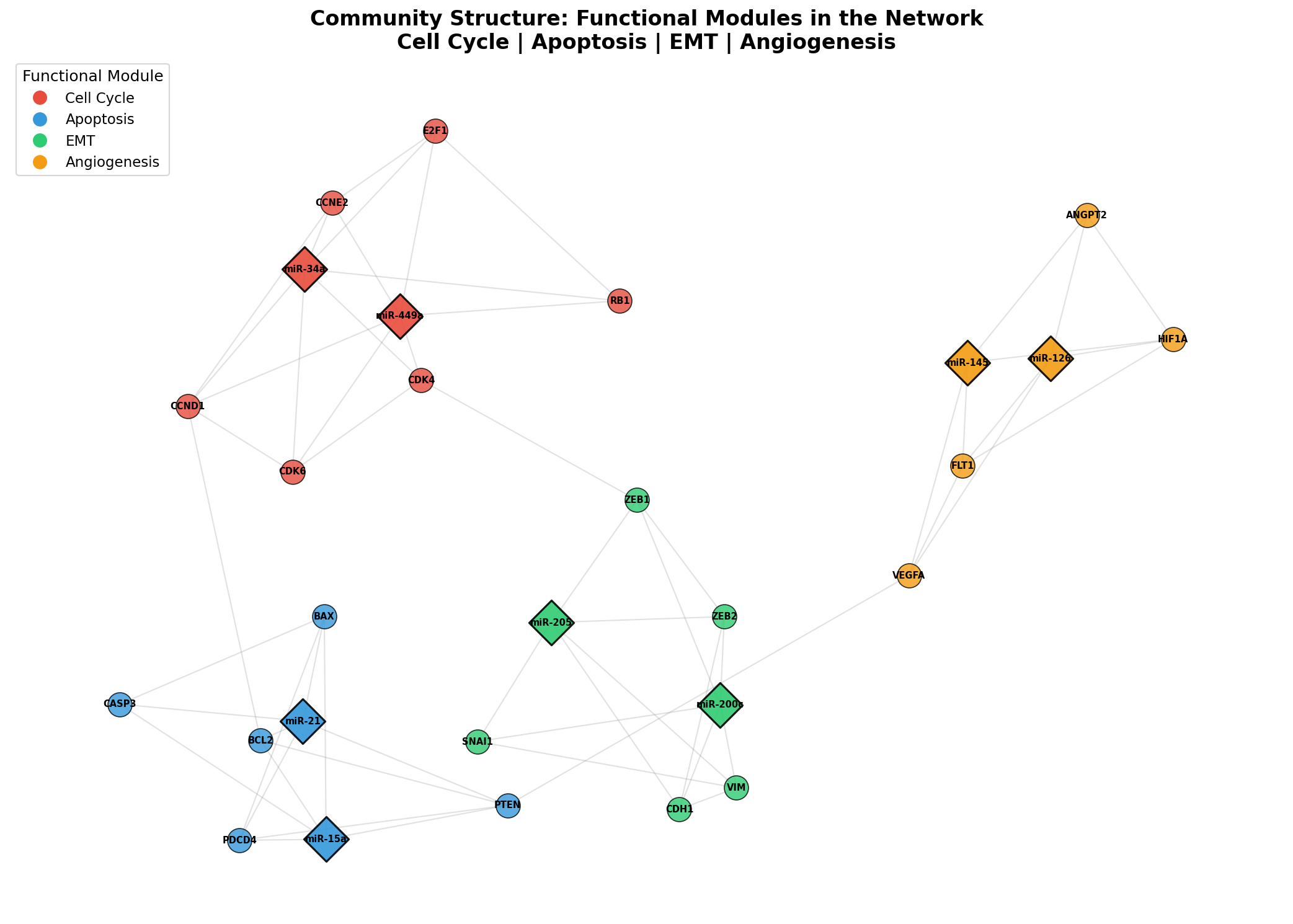
Die Modulanalyse zeigt, dass Krebs kein Einzelgen-Problem ist, sondern ein Netzwerk-Problem. Jedes Modul kann unabhängig dereguliert sein, aber die Cross-Talk-Kanten zwischen Modulen bedeuten, dass die Deregulation eines Moduls auf andere übergreifen kann. Die EMT-Aktivierung (Metastasierung) kann die Angiogenese mitaktivieren — und beide werden von verschiedenen miRNAs gesteuert.
Kapitel 4: Die Stärke der Verbindung — Gewichtete Kanten
Nicht jede Interaktion ist gleich stark. Die Korrelationsstärke zwischen miRNA und Target variiert: Manche Interaktionen sind hochkonsistent über viele Studien validiert, andere nur in einzelnen Experimenten nachgewiesen. Der gewichtete Netzwerk-Graph zeigt diese Evidenzstärke durch Kantendicke und Farbe.
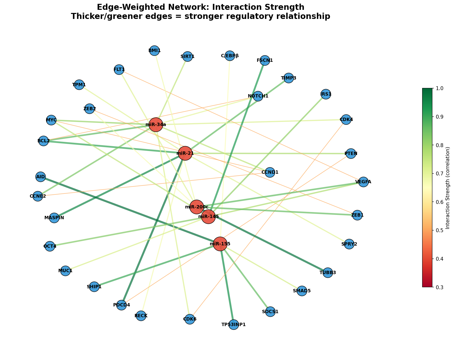
Das gewichtete Netzwerk hilft bei der Priorisierung: Für die experimentelle Validierung konzentriert man sich auf die stärksten Kanten (dickste grüne Linien). Schwache Kanten (dünn, rötlich) sind Hypothesen, die weiterer Bestätigung bedürfen. In der Praxis filtert man das Netzwerk oft auf Kanten mit |Korrelation| > 0.7, um ein übersichtlicheres High-Confidence-Netzwerk zu erhalten.
Kapitel 5: Wer kontrolliert wen? — Zentralitätsmaße
Der Grad ist nur ein Zentralitätsmaß von vielen. Die Betweenness-Zentralität misst, wie oft ein Knoten auf dem kürzesten Pfad zwischen zwei anderen Knoten liegt. Ein Knoten mit hoher Betweenness ist ein Gatekeeper — er kontrolliert den Informationsfluss im Netzwerk, auch wenn er selbst nicht die meisten Verbindungen hat.
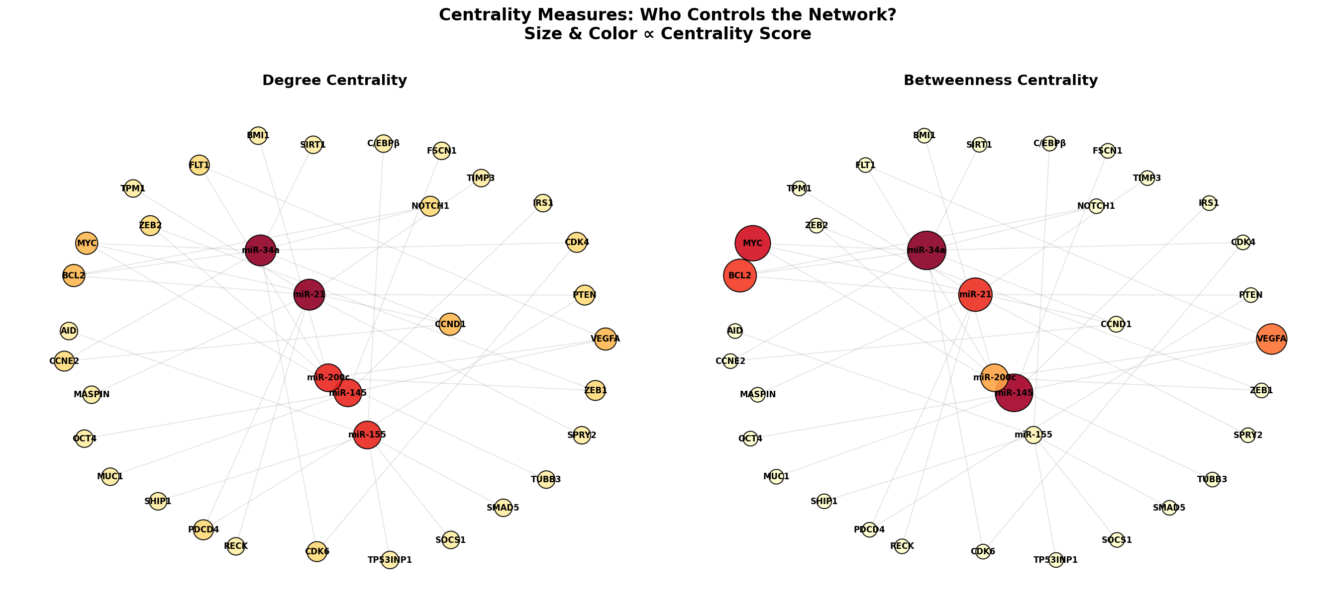
Der Vergleich enthüllt verborgene Schlüsselspieler: Gene, die wenige direkte Verbindungen haben, aber als Brücken zwischen Modulen fungieren. Diese Gatekeeper sind therapeutisch besonders interessant, weil ihre Inhibition nicht nur ein Modul, sondern den Informationsfluss zwischen Modulen unterbricht. In der Systembiologie heißt das: Die wichtigsten Knoten sind nicht immer die größten.
Kapitel 6: Normal vs. Tumor — Das Netzwerk im Krankheitszustand
Die eigentliche Detektivarbeit beginnt, wenn man zwei Netzwerke vergleicht: das normale Gewebe und den Tumor. Im Tumor sind miRNAs dereguliert, neue Targets werden freigeschaltet, und das Netzwerk wird komplexer. Der Vergleich zeigt, was sich verändert hat — und damit, was den Krebs möglicherweise treibt.
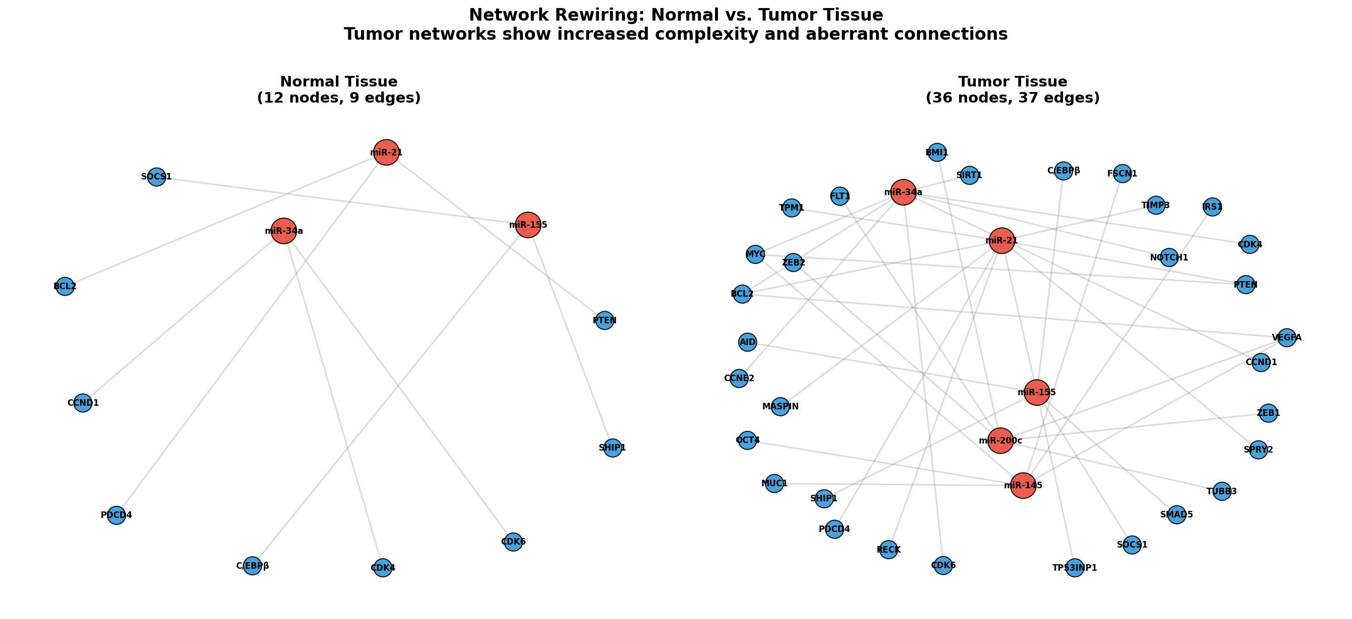
Der direkte Vergleich zeigt das Ausmaß der Netzwerk-Rewiring im Tumor: Neue Kanten entstehen, bestehende werden verstärkt oder geschwächt. Im Normalgewebe ist das Netzwerk schlank und reguliert — im Tumor wird es chaotisch und redundant. Diese Rewiring-Analyse ist ein aktives Forschungsfeld: Differentielle Netzwerkanalyse identifiziert nicht einzelne deregulierte Gene, sondern deregulierte Beziehungen.
Epilog: Das Netzwerk als Denkmodell
Netzwerk-Graphen transformieren die Art, wie wir über Biologie denken. Statt einzelner Gene betrachten wir Systeme. Statt linearer Signalwege sehen wir verwobene Netzwerke mit Redundanz, Modulen und Gatekeepers. Für die Krebsforschung bedeutet das: Die Therapie der Zukunft zielt nicht auf einzelne Gene, sondern auf Netzwerk-Schwachstellen — und der Graph zeigt uns, wo sie liegen.
Zitationen
- Barabási, A.-L. & Oltvai, Z. N. (2004). Network biology: understanding the cell's functional organization. Nature Reviews Genetics, 5(2), 101-113.
- Hsu, S.-D. et al. (2014). miRTarBase update 2014: an information resource for experimentally validated miRNA-target interactions. Nucleic Acids Research, 42(D1), D78-D85.
- Zhang, B. & Horvath, S. (2005). A general framework for weighted gene co-expression network analysis. Statistical Applications in Genetics and Molecular Biology, 4(1), Article 17.
- Csermely, P. et al. (2013). Structure and dynamics of molecular networks: A novel paradigm of drug discovery. Pharmacology & Therapeutics, 138(3), 333-408.
- Yu, H. et al. (2007). The importance of bottlenecks in protein networks: Correlation with gene essentiality and expression dynamics. PLoS Computational Biology, 3(4), e59.
Fazit
Netzwerk-Graphen sind nicht nur Visualisierungen — sie sind analytische Werkzeuge der Systembiologie. Sie identifizieren Hubs (therapeutische Targets), Module (funktionelle Programme), Gatekeepers (Cross-Talk-Controller) und Rewiring (Krankheitsmechanismen). Für die miRNA-Forschung im Speziellen zeigen sie, warum eine einzelne miRNA einen so großen biologischen Effekt haben kann: Sie kontrolliert ein ganzes Subnetzwerk, nicht nur ein einzelnes Gen.
Dokumentation
| Parameter | Wert |
|---|---|
| Hub-miRNAs | miR-21, miR-155, miR-34a, miR-145, miR-200c |
| Target-Datenbank | miRTarBase / TargetScan (validiert) |
| Layout-Algorithmus | Spring Layout (Fruchterman-Reingold) |
| Zentralitätsmaße | Degree, Betweenness |
| Module | Zellzyklus, Apoptose, EMT, Angiogenese |
| Vergleich | Normal vs. Tumor (Netzwerk-Rewiring) |
| Visualisierung | NetworkX + matplotlib (Python) |
Prologue: The Map of Regulators
Genes do not work alone. Every gene is part of a network of regulators, targets, and feedback loops. In cancer biology, it is primarily miRNAs that function as master regulators: A single miRNA can simultaneously control hundreds of target genes. But how do you make these invisible relationships visible? The answer: Network graphs — mathematical structures where nodes represent molecules and edges represent interactions.
In this story, we construct a miRNA-target network for breast cancer and reveal step by step who the control centers are, which modules cooperate, and how the network changes in tumors.
Chapter 1: The Network Emerges — miRNAs and Their Targets
Our starting point: Five hub miRNAs that play central roles in breast cancer biology — miR-21, miR-155, miR-34a, miR-145, and miR-200c. Each regulates a specific group of target genes. The network edges represent experimentally validated miRNA-target interactions from databases like miRTarBase and TargetScan.
The first plot shows the big picture: Red diamonds are miRNAs, blue circles are target genes. The spatial arrangement (spring layout) places strongly connected nodes closer together. It immediately becomes visible which genes are regulated by multiple miRNAs simultaneously — these are the convergence points of the network.
The basic network already reveals an important insight: miRNA regulation is not one-to-one but many-to-many. miR-21 regulates 8 targets, but BCL2 is regulated by both miR-21 and miR-34a. This redundancy makes the network robust — the loss of a single miRNA is compensated by others.
Chapter 2: The Control Centers — Degree-Weighted Networks
Not all nodes are equally important. A node's degree — the number of its connections — is a measure of its influence. Nodes with many connections are called hubs. In biological networks, the degree distribution often follows a power law: Few hubs have extremely many connections, while the majority of nodes have only few.
Hub analysis has direct therapeutic relevance: If a single miRNA simultaneously suppresses 8 tumor suppressor genes (like miR-21), then inhibiting this miRNA is more efficient than activating each individual target. This is the principle of anti-miR therapy — and the network graph shows why it works.
Chapter 3: Functional Modules — Together Rather Than Alone
Biological networks are not randomly wired — they organize into modules: groups of nodes that are strongly connected internally and weakly connected externally. Each module represents a biological function. In our network, we identify four modules: Cell Cycle (red), Apoptosis (blue), Epithelial-Mesenchymal Transition (EMT) (green), and Angiogenesis (orange).
Module analysis shows that cancer is not a single-gene problem but a network problem. Each module can be independently deregulated, but cross-talk edges between modules mean that deregulation of one module can spread to others. EMT activation (metastasis) can co-activate angiogenesis — and both are controlled by different miRNAs.
Chapter 4: The Strength of Connection — Weighted Edges
Not every interaction is equally strong. Correlation strength between miRNA and target varies: Some interactions are highly consistently validated across many studies, others demonstrated only in single experiments. The weighted network graph shows this evidence strength through edge thickness and color.
The weighted network helps with prioritization: For experimental validation, one focuses on the strongest edges (thickest green lines). Weak edges (thin, reddish) are hypotheses requiring further confirmation. In practice, networks are often filtered to edges with |correlation| > 0.7 to obtain a cleaner high-confidence network.
Chapter 5: Who Controls Whom? — Centrality Measures
Degree is just one centrality measure of many. Betweenness centrality measures how often a node lies on the shortest path between two other nodes. A node with high betweenness is a gatekeeper — it controls information flow in the network, even if it does not have the most connections itself.
The comparison reveals hidden key players: Genes with few direct connections but functioning as bridges between modules. These gatekeepers are therapeutically particularly interesting because their inhibition disrupts not just one module but the information flow between modules. In systems biology terminology: The most important nodes are not always the largest.
Chapter 6: Normal vs. Tumor — The Network in Disease
The real detective work begins when comparing two networks: normal tissue and tumor. In tumors, miRNAs are deregulated, new targets are unlocked, and the network becomes more complex. The comparison shows what has changed — and thus what potentially drives the cancer.
The direct comparison shows the extent of network rewiring in tumors: New edges emerge, existing ones are strengthened or weakened. In normal tissue, the network is lean and regulated — in tumors, it becomes chaotic and redundant. This rewiring analysis is an active research field: Differential network analysis identifies not individually deregulated genes, but deregulated relationships.
Epilogue: The Network as Mental Model
Network graphs transform how we think about biology. Instead of individual genes, we examine systems. Instead of linear signaling pathways, we see interwoven networks with redundancy, modules, and gatekeepers. For cancer research, this means: Future therapy targets not individual genes but network vulnerabilities — and the graph shows us where they lie.
Citations
- Barabási, A.-L. & Oltvai, Z. N. (2004). Network biology: understanding the cell's functional organization. Nature Reviews Genetics, 5(2), 101-113.
- Hsu, S.-D. et al. (2014). miRTarBase update 2014: an information resource for experimentally validated miRNA-target interactions. Nucleic Acids Research, 42(D1), D78-D85.
- Zhang, B. & Horvath, S. (2005). A general framework for weighted gene co-expression network analysis. Statistical Applications in Genetics and Molecular Biology, 4(1), Article 17.
- Csermely, P. et al. (2013). Structure and dynamics of molecular networks: A novel paradigm of drug discovery. Pharmacology & Therapeutics, 138(3), 333-408.
- Yu, H. et al. (2007). The importance of bottlenecks in protein networks: Correlation with gene essentiality and expression dynamics. PLoS Computational Biology, 3(4), e59.
Conclusion
Network graphs are not just visualizations — they are analytical tools of systems biology. They identify hubs (therapeutic targets), modules (functional programs), gatekeepers (cross-talk controllers), and rewiring (disease mechanisms). For miRNA research specifically, they show why a single miRNA can have such a large biological effect: It controls an entire subnetwork, not just a single gene.
Documentation
| Parameter | Value |
|---|---|
| Hub miRNAs | miR-21, miR-155, miR-34a, miR-145, miR-200c |
| Target database | miRTarBase / TargetScan (validated) |
| Layout algorithm | Spring Layout (Fruchterman-Reingold) |
| Centrality measures | Degree, Betweenness |
| Modules | Cell Cycle, Apoptosis, EMT, Angiogenesis |
| Comparison | Normal vs. Tumor (network rewiring) |
| Visualization | NetworkX + matplotlib (Python) |