Abstract
scanpy ist das Python-Referenzpaket für die Analyse von Single-Cell-RNA-Seq-Daten (scRNA-Seq). Es deckt die gesamte Pipeline ab – von der Qualitätskontrolle und Normalisierung über Dimensionsreduktion (PCA, UMAP, t-SNE) und Clustering (Leiden, Louvain) bis zur Identifikation von Markergenen und Zelltyp-Annotation. Auf Basis des AnnData-Objekts als zentraler Datenstruktur integriert scanpy sich nahtlos mit scvi-tools, CellRank und dem gesamten scverse-Ökosystem. Für Bioinformatik-Teams, die große Single-Cell-Datensätze (10&sup5;–10&sup7; Zellen) effizient verarbeiten müssen, ist scanpy die erste Wahl im Python-Stack.
Typisches Projektszenario
Ein Immunologie-Labor untersucht die Heterogenität von CD8+ T-Zellen in Tumorgewebe (TILs) aus 8 Melanom-Patienten. Pro Patient werden ~5.000 Zellen per 10x Genomics Chromium erfasst (40.000 Zellen total). Die CellRanger-Ausgabe (gefilterte Feature-Barcode-Matrix) wird in scanpy geladen. Ziel: Subpopulationen identifizieren (naïv, effector, exhausted, progenitor exhausted), deren Marker definieren und die klonale Expansion über TCR-Daten mit dem Erschöpfungsphänotyp verbinden.
Welches Problem löst scanpy?
- Sparse, hochdimensionale Daten: Eine typische scRNA-Seq-Matrix hat 20.000 Gene × 40.000 Zellen, wobei >90% der Einträge Null sind (Dropout). scanpy arbeitet nativ mit Sparse-Matrizen (scipy.sparse) und skaliert effizient auf Millionen von Zellen.
- Batch-Effekte zwischen Patienten: Technische und biologische Variabilität überlagern sich. scanpy integriert mit Harmony, scVI, bbknn und anderen Batch-Korrektur-Methoden, um patientenspezifische Effekte zu entfernen, während biologische Variation erhalten bleibt.
- Zelltyp-Identifikation: Die unbekannte Zellzusammensetzung muss aus den Daten selbst erschlossen werden – über Clustering, Markergene und Vergleich mit Referenzatlanten.
Warum Teams scanpy einsetzen
- AnnData-Objekt: Das zentrale Datenobjekt speichert Expressionsmatrix, Zell-Metadaten, Gen-Annotationen, Dimensionsreduktionen und Graphen in einer einzigen Struktur – keine separaten Dateien oder Konvertierungen nötig.
- GPU-Beschleunigung: Über rapids-singlecell können rechenintensive Schritte (PCA, Neighbor-Graphen, UMAP) auf NVIDIA-GPUs ausgeführt werden – 10–100× Speedup.
- Modularer Aufbau: Jeder Analyseschritt ist eine eigenständige Funktion (sc.pp.*, sc.tl.*, sc.pl.*), die das AnnData-Objekt in-place modifiziert – das macht Pipelines reproduzierbar und leicht anpassbar.
- scverse-Integration: squidpy (spatial), scvi-tools (probabilistische Modelle), CellRank (Trajektorien), muon (Multiomics) – alle bauen auf AnnData/scanpy auf.
- Community: >1.500 GitHub-Stars, aktive Entwicklung, umfangreiche Tutorials und ein wachsendes Plugin-Ökosystem.
scanpy-Pipeline im Detail
Die Qualitätskontrolle bildet das Fundament jeder scRNA-Seq-Analyse. scanpy berechnet per-Zell-Metriken (Gene pro Zelle, Counts pro Zelle, Anteil mitochondrialer Reads) über sc.pp.calculate_qc_metrics(). Typische Filter: Zellen mit <200 Genen oder >20% mitochondrialen Reads werden entfernt – erstere sind leere Droplets oder Debris, letztere sterbende Zellen mit Zytoplasma-Verlust. Gene, die in weniger als 3 Zellen exprimiert sind, werden ebenfalls gefiltert.
Die Normalisierung mit sc.pp.normalize_total() (Library-Size-Normalisierung zu 10.000 Counts pro Zelle) gefolgt von sc.pp.log1p() (Log-Transformation) erzeugt die Grundlage für alle nachfolgenden Schritte. Alternativ bietet scvi-tools eine probabilistische Normalisierung, die biologische und technische Varianz trennt.
Die Feature-Selektion mit sc.pp.highly_variable_genes() (typisch: 2.000–4.000 HVGs) reduziert das Rauschen und fokussiert die Analyse auf biologisch informative Gene. Der Seurat-v3-Flavor (flavor='seurat_v3') ist der robusteste Ansatz für UMI-basierte Daten.
Python-Code: scanpy-Pipeline
import scanpy as sc
import numpy as np

sc.settings.verbosity = 2
sc.settings.figdir = './figures/'

# Daten laden (10x CellRanger Output)
adata = sc.read_10x_mtx('./filtered_feature_bc_matrix/',
                         var_names='gene_symbols', cache=True)
adata.var_names_make_unique()

# QC-Metriken + Filtern
adata.var['mt'] = adata.var_names.str.startswith('MT-')
sc.pp.calculate_qc_metrics(adata, qc_vars=['mt'],
                            percent_top=None, inplace=True)
adata = adata[adata.obs.n_genes_by_counts.between(200, 5000) &
              (adata.obs.pct_counts_mt < 20)].copy()

# Normalisierung + Log-Transformation
sc.pp.normalize_total(adata, target_sum=1e4)
sc.pp.log1p(adata)

# Highly Variable Genes
sc.pp.highly_variable_genes(adata, n_top_genes=3000,
                             flavor='seurat_v3')
adata.raw = adata
adata = adata[:, adata.var.highly_variable]

# PCA + Nachbar-Graph + Clustering
sc.pp.scale(adata, max_value=10)
sc.tl.pca(adata, n_comps=50, svd_solver='arpack')
sc.pp.neighbors(adata, n_neighbors=15, n_pcs=30)
sc.tl.leiden(adata, resolution=0.8)

# UMAP + Markergene
sc.tl.umap(adata, min_dist=0.3)
sc.tl.rank_genes_groups(adata, 'leiden', method='wilcoxon')

# Visualisierung
sc.pl.umap(adata, color=['leiden', 'CD8A', 'PDCD1', 'TCF7'],
           save='_til_markers.png')
sc.pl.rank_genes_groups_dotplot(adata, n_genes=5,
                                 save='_markers_dotplot.png')
Beispielausgabe
# Loaded 42,318 cells x 33,694 genes
# Filtered to 38,456 cells (QC)
# 3,000 highly variable genes selected
# PCA: 50 components, 30 used for neighbors
# Leiden clustering: 14 clusters at resolution 0.8

# Top markers per cluster (Wilcoxon):
# Cluster 0: TCF7, LEF1, CCR7, SELL     (naive)
# Cluster 1: GZMB, PRF1, GNLY, NKG7     (effector)
# Cluster 3: PDCD1, HAVCR2, LAG3, TOX   (exhausted)
# Cluster 5: TCF7, PDCD1, SLAMF6        (prog. exhausted)
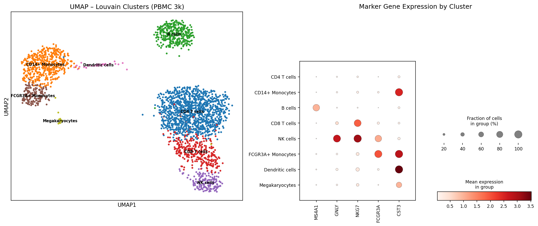
Diagnostische Plots
Vergleich mit Alternativen
| Merkmal | scanpy | Seurat (R) | scvi-tools |
|---|---|---|---|
| Sprache | Python | R | Python (PyTorch) |
| Datenobjekt | AnnData | SeuratObject | AnnData |
| Max. Zellzahl | >107 | ~106 | >107 |
| GPU-Support | Ja (rapids) | Nein (nativ) | Ja (PyTorch) |
| Batch-Korrektur | bbknn, Harmony | CCA, RPCA, Harmony | scVI (probabilistisch) |
| Normalisierung | Shift-Log, scran | LogNormalize, SCTransform | scVI (latent) |
| Clustering | Leiden, Louvain | Louvain, Leiden | Über scanpy |
Statistische Vertiefung
Die Leiden-Algorithmus-Implementierung in scanpy nutzt den modularity-basierten Community-Detection-Ansatz auf dem k-Nearest-Neighbor-Graphen. Der Resolution-Parameter γ steuert die Granularität: γ=0.5 liefert wenige große Cluster, γ=2.0 viele kleine. Die Wahl von γ ist kritisch und sollte über Silhouette-Scores oder biologische Marker validiert werden – nicht blind optimiert. Der Leiden-Algorithmus garantiert im Gegensatz zu Louvain, dass alle resultierenden Communities zusammenhängend sind.
Die UMAP-Embeddings sind Visualisierungen, keine quantitativen Analysetools. Absolute Distanzen zwischen Clustern in der UMAP sind nicht interpretierbar – nur die relative Nachbarschaft ist informativ. Zwei Cluster, die im UMAP weit auseinander liegen, können im hochdimensionalen Raum durchaus ähnlich sein. Alle quantitativen Analysen (DE-Tests, Trajektorie-Inferenz) sollten auf den PCA-Daten oder dem Nachbar-Graphen basieren, nicht auf UMAP-Koordinaten.
Der Wilcoxon-Rangsummentest in rank_genes_groups() testet für jedes Gen, ob es in einem Cluster höher exprimiert ist als in allen anderen Zellen. Der Test ist nicht-parametrisch und robust gegen die Verletzung von Normalverteilungsannahmen in scRNA-Seq-Daten. Die Benjamini-Hochberg-Korrektur kontrolliert die False Discovery Rate. Alternative: der t-Test mit Overestimation-Correction (method='t-test_overestim_var') ist konservativer und vermeidet falsch-positive Marker bei großen Zellzahlen.
Zitationen
- Wolf FA, Angerer P, Theis FJ (2018). “SCANPY: large-scale single-cell gene expression data analysis.” Genome Biology, 19, 15.
- Virshup I et al. (2023). “The scverse project provides a computational framework for single-cell omics data analysis.” Nature Biotechnology, 41, 604–606.
- Traag VA, Waltman L, van Eck NJ (2019). “From Louvain to Leiden: guaranteeing well-connected communities.” Scientific Reports, 9, 5233.
Fazit
scanpy ist das Arbeitspferd der Single-Cell-Analyse im Python-Ökosystem. Es vereint Geschwindigkeit (Sparse-Matrizen, GPU-Support), Modularität (scverse-Plugins) und eine aktive Community. Für Teams, die bereits in Python arbeiten, ist scanpy die natürliche Wahl gegenüber Seurat. Limitierungen: (1) Die Qualität der Ergebnisse hängt stark von der Parameterwahl ab (n_neighbors, resolution, n_pcs). (2) Die Log-Normalisierung ist statistisch suboptimal – probabilistische Methoden (scVI) liefern bessere latente Repräsentationen. (3) Zelltyp-Annotation erfordert nach wie vor Expertenwissen und manuelle Kuration – automatisierte Tools (CellTypist, scArches) können unterstützen, aber nicht ersetzen.
Dokumentation
Abstract
scanpy is the Python reference package for single-cell RNA-Seq (scRNA-Seq) data analysis. It covers the entire pipeline—from quality control and normalization through dimensionality reduction (PCA, UMAP, t-SNE) and clustering (Leiden, Louvain) to marker gene identification and cell type annotation. Built on the AnnData object as the central data structure, scanpy integrates seamlessly with scvi-tools, CellRank, and the broader scverse ecosystem. For bioinformatics teams needing to efficiently process large single-cell datasets (105–107 cells), scanpy is the first choice in the Python stack.
Typical Project Scenario
An immunology lab investigates the heterogeneity of CD8+ T cells in tumor tissue (TILs) from 8 melanoma patients. ~5,000 cells per patient are captured via 10x Genomics Chromium (40,000 cells total). CellRanger output (filtered feature-barcode matrix) is loaded into scanpy. Goal: identify subpopulations (naive, effector, exhausted, progenitor exhausted), define their markers, and link clonal expansion via TCR data with the exhaustion phenotype.
What Problem Does scanpy Solve?
- Sparse, high-dimensional data: A typical scRNA-Seq matrix has 20,000 genes × 40,000 cells, with >90% of entries being zero (dropout). scanpy works natively with sparse matrices (scipy.sparse) and scales efficiently to millions of cells.
- Batch effects between patients: Technical and biological variability overlap. scanpy integrates with Harmony, scVI, bbknn, and other batch correction methods to remove patient-specific effects while preserving biological variation.
- Cell type identification: The unknown cell composition must be inferred from the data itself—through clustering, marker genes, and comparison with reference atlases.
Why Teams Choose scanpy
- AnnData object: The central data object stores expression matrix, cell metadata, gene annotations, dimensionality reductions, and graphs in a single structure—no separate files or conversions needed.
- GPU acceleration: Via rapids-singlecell, compute-intensive steps (PCA, neighbor graphs, UMAP) can run on NVIDIA GPUs—10–100× speedup.
- Modular design: Each analysis step is a standalone function (sc.pp.*, sc.tl.*, sc.pl.*) that modifies the AnnData object in-place—making pipelines reproducible and easily customizable.
- scverse integration: squidpy (spatial), scvi-tools (probabilistic models), CellRank (trajectories), muon (multiomics)—all build on AnnData/scanpy.
- Community: >1,500 GitHub stars, active development, extensive tutorials, and a growing plugin ecosystem.
scanpy Pipeline in Detail
Quality control forms the foundation of every scRNA-Seq analysis. scanpy computes per-cell metrics (genes per cell, counts per cell, mitochondrial read fraction) via sc.pp.calculate_qc_metrics(). Typical filters: cells with <200 genes or >20% mitochondrial reads are removed—the former are empty droplets or debris, the latter dying cells with cytoplasm loss. Genes expressed in fewer than 3 cells are also filtered.
Normalization with sc.pp.normalize_total() (library-size normalization to 10,000 counts per cell) followed by sc.pp.log1p() (log transformation) creates the foundation for all subsequent steps. Alternatively, scvi-tools offers probabilistic normalization that separates biological and technical variance.
Feature selection with sc.pp.highly_variable_genes() (typically 2,000–4,000 HVGs) reduces noise and focuses analysis on biologically informative genes. The Seurat-v3 flavor (flavor='seurat_v3') is the most robust approach for UMI-based data.
Python Code: scanpy Pipeline
import scanpy as sc
import numpy as np

sc.settings.verbosity = 2
sc.settings.figdir = './figures/'

# Load data (10x CellRanger output)
adata = sc.read_10x_mtx('./filtered_feature_bc_matrix/',
                         var_names='gene_symbols', cache=True)
adata.var_names_make_unique()

# QC metrics + filtering
adata.var['mt'] = adata.var_names.str.startswith('MT-')
sc.pp.calculate_qc_metrics(adata, qc_vars=['mt'],
                            percent_top=None, inplace=True)
adata = adata[adata.obs.n_genes_by_counts.between(200, 5000) &
              (adata.obs.pct_counts_mt < 20)].copy()

# Normalization + log transformation
sc.pp.normalize_total(adata, target_sum=1e4)
sc.pp.log1p(adata)

# Highly variable genes
sc.pp.highly_variable_genes(adata, n_top_genes=3000,
                             flavor='seurat_v3')
adata.raw = adata
adata = adata[:, adata.var.highly_variable]

# PCA + neighbor graph + clustering
sc.pp.scale(adata, max_value=10)
sc.tl.pca(adata, n_comps=50, svd_solver='arpack')
sc.pp.neighbors(adata, n_neighbors=15, n_pcs=30)
sc.tl.leiden(adata, resolution=0.8)

# UMAP + marker genes
sc.tl.umap(adata, min_dist=0.3)
sc.tl.rank_genes_groups(adata, 'leiden', method='wilcoxon')

# Visualization
sc.pl.umap(adata, color=['leiden', 'CD8A', 'PDCD1', 'TCF7'],
           save='_til_markers.png')
sc.pl.rank_genes_groups_dotplot(adata, n_genes=5,
                                 save='_markers_dotplot.png')
Example Output
# Loaded 42,318 cells x 33,694 genes
# Filtered to 38,456 cells (QC)
# 3,000 highly variable genes selected
# PCA: 50 components, 30 used for neighbors
# Leiden clustering: 14 clusters at resolution 0.8

# Top markers per cluster (Wilcoxon):
# Cluster 0: TCF7, LEF1, CCR7, SELL     (naive)
# Cluster 1: GZMB, PRF1, GNLY, NKG7     (effector)
# Cluster 3: PDCD1, HAVCR2, LAG3, TOX   (exhausted)
# Cluster 5: TCF7, PDCD1, SLAMF6        (prog. exhausted)
Diagnostic Plots
Comparison with Alternatives
| Feature | scanpy | Seurat (R) | scvi-tools |
|---|---|---|---|
| Language | Python | R | Python (PyTorch) |
| Data object | AnnData | SeuratObject | AnnData |
| Max cells | >107 | ~106 | >107 |
| GPU support | Yes (rapids) | No (native) | Yes (PyTorch) |
| Batch correction | bbknn, Harmony | CCA, RPCA, Harmony | scVI (probabilistic) |
| Normalization | Shift-log, scran | LogNormalize, SCTransform | scVI (latent) |
| Clustering | Leiden, Louvain | Louvain, Leiden | Via scanpy |
Statistical Deep Dive
The Leiden algorithm implementation in scanpy uses modularity-based community detection on the k-nearest-neighbor graph. The resolution parameter γ controls granularity: γ=0.5 yields few large clusters, γ=2.0 many small ones. The choice of γ is critical and should be validated via silhouette scores or biological markers—not blindly optimized. The Leiden algorithm guarantees, unlike Louvain, that all resulting communities are connected.
UMAP embeddings are visualizations, not quantitative analysis tools. Absolute distances between clusters in UMAP are not interpretable—only relative neighborhood is informative. Two clusters far apart in UMAP may well be similar in high-dimensional space. All quantitative analyses (DE tests, trajectory inference) should be based on PCA data or the neighbor graph, not UMAP coordinates.
The Wilcoxon rank-sum test in rank_genes_groups() tests for each gene whether it is more highly expressed in one cluster than in all other cells. The test is non-parametric and robust against violations of normality assumptions in scRNA-Seq data. Benjamini-Hochberg correction controls the false discovery rate. Alternative: the t-test with overestimation correction (method='t-test_overestim_var') is more conservative and avoids false positive markers with large cell numbers.
Citations
- Wolf FA, Angerer P, Theis FJ (2018). “SCANPY: large-scale single-cell gene expression data analysis.” Genome Biology, 19, 15.
- Virshup I et al. (2023). “The scverse project provides a computational framework for single-cell omics data analysis.” Nature Biotechnology, 41, 604–606.
- Traag VA, Waltman L, van Eck NJ (2019). “From Louvain to Leiden: guaranteeing well-connected communities.” Scientific Reports, 9, 5233.
Conclusion
scanpy is the workhorse of single-cell analysis in the Python ecosystem. It combines speed (sparse matrices, GPU support), modularity (scverse plugins), and an active community. For teams already working in Python, scanpy is the natural choice over Seurat. Limitations: (1) Result quality heavily depends on parameter choices (n_neighbors, resolution, n_pcs). (2) Log normalization is statistically suboptimal—probabilistic methods (scVI) provide better latent representations. (3) Cell type annotation still requires expert knowledge and manual curation—automated tools (CellTypist, scArches) can assist but not replace human judgment.